(d). Topographic Maps

Introduction

A topographic map is a detailed and accurate two-dimensional representation of natural and human-made features on the Earth's surface. These maps are used for a number of applications, from camping, hunting, fishing, and hiking to urban planning, resource management, and surveying. The most distinctive characteristic of a topographic map is that the three-dimensional shape of the Earth's surface is modeled by the use of contour lines. Contours are imaginary lines that connect locations of similar elevation. Contours make it possible to represent the height of mountains and steepness of slopes on a two-dimensional map surface. Topographic maps also use a variety of symbols to describe both natural and human made features such as roads, buildings, quarries, lakes, streams, and vegetation.

Topographic maps produced by the Canadian National Topographic System (NTS) are generally available in two different scales: 1:50,000 and 1:250,000. Maps with a scale of 1:50,000 are relatively large-scale covering an area approximately 1000 square kilometers. At this scale, features as small as a single home can be shown. The smaller scale 1:250,000 topographic map is more of a general purpose reconnaissance-type map. A map of this scale covers the same area of land as sixteen 1:50,000 scale maps.

In the United States, topographic maps have been made by the United States Geological Survey (USGS) since 1879. Topographic coverage of the United States is available at scales of 1:24,000, 1:25,000 (metric), 1:62,250, 1:63,360 (Alaska only), 1:100,000 and 1:250,000.

 

Topographic Map Symbols

Topographic maps use symbols to represent natural and human constructed features found in the environment. The symbols used to represent features can be of three types: points, lines, and polygons. Points are used to depict features like bridges and buildings. Lines are used to graphically illustrate features that are linear. Some common linear features include roads, railways, and rivers. However, we also need to include representations of area, in the case of forested land or cleared land; this is done through the use of color.

The set of symbols used on Canadian National Topographic System (NTS) maps has been standardized to simplify the map construction process. A description of the complete set of symbols available can be found in a published guide titled: Standards and Specifications for Polychrome Maps. This guide guarantees uniform illustration of surface features on both 1:50 000 and 1:250 000 topographic maps. Despite the existence of this guide, we can find that some topographic maps may use different symbols to depict a feature. This occurs because the symbols used are graphically refined over time - as a result the Standards and Specifications for Polychrome Maps guide is always under revision.

The tables below describe some of the common symbols used on Canadian National Topographic System maps (source: Centre for Topographic Information, Natural Resources Canada). See the following link for the symbols commonly used on USGS topographic maps.

Transportation Features - Roads and Trails

Feature Name	Symbol
Road - hard surface, all season
Road - hard surface, all season
Road - loose or stabilized surface, all season
Road - loose surface, dry weather
Rapid transit route, road
Road under construction
Vehicle track or winter road
Trail or portage
Traffic circle
Highway route number

 

Transportation Features - Railways and Airports

Feature Name	Symbol
Railway - multiple track
Railway - single track
Railway sidings
Railway - rapid transit
Railway - under construction
Railway - abandoned
Railway on road
Railway station
Airfield; Heliport
Airfield, position approximate
Airfield runways; paved, unpaved

 

Other Transportation Features - Tunnels, Bridges, etc.

Feature Name	Symbol
Tunnel; railway, road
Bridge
Bridge; swing, draw, lift
Footbridge
Causeway
Ford
Cut
Embankment
Snow shed
Barrier or gate

 

Hydrographic Features - Human Made

Feature Name	Symbol
Lock
Dam; large, small
Dam carrying road
Footbridge
Ferry Route
Pier; Wharf; Seawall
Breakwater
Slip; Boat ramp; Drydock
Canal; navigable or irrigation
Canal, abandoned
Shipwreck, exposed
Crib or abandoned bridge pier
Submarine cable
Seaplane anchorage; Seaplane base

 

Hydrographic Features - Naturally Occurring

Feature Name	Symbol
Falls
Rapids
Direction of flow arrow
Dry river bed
Stream - intermittent
Sand in Water or Foreshore Flats
Rocky ledge, reef
Flooded area
Marsh, muskeg
Swamp
Well, water or brine; Spring
Rocks in water or small islands
Water elevation

 

Terrain Features - Elevation

Feature Name	Symbol
Horizontal control point; Bench mark with elevation
Precise elevation
Contours; index, intermediate
Depression contours

 

Terrain Features - Geology and Geomorphology

Feature Name	Symbol
Cliff or escarpment
Esker
Pingo
Sand
Moraine
Quarry
Cave

 

Terrain Features - Land Cover

Feature Name	Symbol
Wooded area
Orchard
Vineyard

 

Human Activity Symbols - Recreation

Feature Name	Symbol
Sports track
Swimming pool
Stadium
Golf course
Golf driving range
Campground; Picnic site
Ski area, ski jump
Rifle range with butts
Historic site or point of interest; Navigation light
Aerial cableway, ski lift

 

Human Activity Symbols - Agriculture and Industry

Feature Name	Symbol
Silo
Elevator
Greenhouse
Wind-operated device; Mine
Landmark object (with height); tower, chimney, etc.
Oil or natural gas facility
Pipeline, multiple pipelines, control valve
Pipeline, underground multiple pipelines, underground
Electric facility
Power transmission line multiple lines
Telephone line
Fence
Crane, vertical and horizontal
Dyke or levee
Firebreak
Cut line

 

Human Activity Symbols - Buildings

Feature Name	Symbol
School; Fire station; Police station
Church; Non-Christian place of worship; Shrine
Building
Service centre
Customs post
Coast Guard station
Cemetery
Ruins
Fort

 

Contour Lines

Topographic maps can describe vertical information through the use of contour lines (contours). A contour line is an isoline that connects points on a map that have the same elevation. Contours are often drawn on a map at a uniform vertical distance. This distance is called the contour interval. The map in the Figure 2d-1 shows contour lines with an interval of 100 feet. Note that every fifth brown contour lines is drawn bold and has the appropriate elevation labeled on it. These contours are called index contours. On Figure 2d-1 they represent elevations of 500, 1000, 1500, 2000 feet and so on. The interval at which contours are drawn on a map depends on the amount of the relief depicted and the scale of the map.

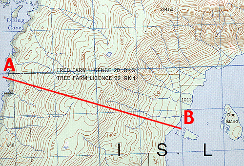
Figure 2d-1: Portion of the "Tofino" 1:50,000 National Topographic Series of Canada map. The brown lines drawn on this map are contour lines. Each line represents a vertical increase in elevation of 100 feet. The bold brown contour lines are called index contours. The index contours are labeled with their appropriate elevation which increases at a rate of 500 feet. Note the blue line drawn to separate water from land represents an elevation of 0 feet or sea-level.

 

Contour lines provide us with a simple effective system for describing landscape configuration on a two-dimensional map. The arrangement, spacing, and shape of the contours provide the user of the map with some idea of what the actual topographic configuration of the land surface looks like. Contour intervals the are spaced closely together describe a steep slope. Gentle slopes are indicated by widely spaced contours. Contour lines that V upwards indicate the presence of a river valley. Ridges are shown by contours that V downwards.

 

Topographic Profiles

A topographic profile is a two-dimensional diagram that describes the landscape in vertical cross-section. Topographic profiles are often created from the contour information found on topographic maps. The simplest way to construct a topographic profile is to place a sheet of blank paper along a horizontal transect of interest. From the map, the elevation of the various contours is transferred on to the edge of the paper from one end of the transect to the other. Now on a sheet of graph paper use the x-axis to represent the horizontal distance covered by the transect. The y-axis is used to represent the vertical dimension and measures the change in elevation along the transect. Most people exaggerate the measure of elevation on the y-axis to make changes in relief stand out. Place the beginning of the transect as copied on the piece of paper at the intersect of the x and y-axis on the graph paper. The contour information on the paper's edge is now copied onto the piece of graph paper. Figure 2d-2 shows a topographic profile drawn from the information found on the transect A-B above.

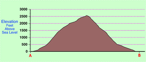
Figure 1d-2: The following topographic profile shows the vertical change in surface elevation along the transect AB from Figure 1d-1. A vertical exaggeration of about 4.2 times was used in the profile (horizontal scale = 1:50,000, vertical scale = 1:12,000 and vertical exaggeration = horizontal scale/vertical scale).

 

Military Grid Reference System and Map Location

Two rectangular grid systems are available on topographic maps for identifying the location of points. These systems are the Universal Transverse Mercator (UTM) grid system and the Military Grid Reference System. The Military Grid Reference System is a simplified form of Universal Transverse Mercator grid system and it provides a very quick and easy method of referencing a location on a topographic map. On a topographic maps with a scale 1:50,000 and larger, the Military Grid Reference System is superimposed on the surface of map as blue colored series of equally spaced horizontal and vertical lines. Identifying numbers for each of these lines is found along the map's margin. Each identifying number consists of two digits which range from a value of 00 to 99 (Figure 2d-3). Each individual square in the grid system represents a distance of a 1000 by 1000 meters and the total size of the grid is 100,000 by 100,000 meters.

One problem associated with the Military Grid Reference System is the fact that reference numbers must be repeated every 100,000 meters. To overcome this difficulty, a method was devised to identify each 100,000 by 100,000 meter grid with two identifying letters which are printed in blue on the border of all topographic maps (note some maps may show more than one grid). When making reference to a location with the Military Grid Reference System identifying letters are always given before the horizontal and vertical coordinate numbers.

Figure 2d-3: Portion of a Military Grid Reference System found on a topographic map. Coordinates on this system are based on a X (horizontal increasing from left to right) and Y (vertical increasing from bottom to top) system. The symbol depicting a church is located in the square 9194. Note that the value along the X-axis (easting) is given first followed by the value on the Y-axis (northing). (Source: Centre for Topographic Information, Natural Resources Canada).

 

Each individual square in the Military Grid Reference System can be further divided into 100 smaller squares (ten by ten). This division allows us to calculate the location of an object to within 100 meters. Figure 1d-4 indicates that the church is six tenths of the way between lines 91 and 92, and four tenths of the way between lines 94 and 95. Using these values, we can state that the easting as being 916 and the northing as 944. By convention, these two numbers are combined into a coordinate reference of 916944.

Figure 2d-4: Further determination of the location of the church described in Figure 2d-3. Using the calibrated ruler we can now suggest the location of the church to be 916 on the X-axis and 944 on the Y-axis. Note that the location reference always has an even number of digits, with the three digits representing the easting and the second three the northing. (Source: Centre for Topographic Information, Natural Resources Canada).

 

Study Guide

Additional Readings