(g). Inferential Statistics: Comparison of Sample Means

Introduction

In Physical Geography it is often necessary to test whether two samples of the same natural event are statistically distinct under different conditions. For example, a research scientist may want to determine if rainfall from convective storms differs in its intensity in rural and adjacent urban landscapes. Information from this investigation can then be used to test theories concerning the influence of the urban landscape on the development of thunderstorms. Further, this type of hypothesis testing changes our general comprehension in Physical Geography from simple description to process oriented understanding. A number of inferential statistical procedures have been developed to carry out this process. We will examine two of the most popular statistical techniques available to researchers.

 

Mann-Whitney U test

In research work it is often necessary to test whether two samples of the same phenomenon are statistically different. One test that is particularly useful for this type of test situation is the Mann-Whitney U test. This technique is non-parametric or 'distribution-free' in nature. Non-parametric methods are particularly suited to data that are not normally distributed.

 

Setting up the Null Hypothesis

This is the first stage of any statistical analysis and states the hypothesis that is to be tested. This is the assumption that will be maintained unless the data provide significant evidence to discredit it. The null hypothesis is denoted symbolically as H0. For our example, the null hypothesis would be:

H0 : there is no difference in precipitation levels between urban and adjacent rural areas.

It is also necessary to state the alternative hypothesis (H1). In this case the alternative might be:

H1 : there is an increase in precipitation levels in urban areas relative to adjacent rural areas because of the heating differences of the two surface types (the urban area heats up more and has increased convective uplift).

 

 

Calculation

To calculate the U-statistic, the values for both sets of samples are ranked together in an ascending fashion. When ties occur, the mean rank of all the scores involved in the tie is entered for those observations. The rank values for each set of observations are then summed separately to determine the following values:

S r1 and S r2

These values are then entered in the formulae shown under Table 3g-1 for the calculation of U and U1.

 

Table 3g-1: Analysis of convective precipitation levels per storm event (mm of rain) between urban and rural areas using the Mann-Whitney U test.

Urban (n1)	Rural (n2)	Rank (n1)	Rank (n2)
28	14	26	5
27	20	25	13.5
33	16	28	8.5
23	13	20	2.5
24	18	23	11
17	21	10	16
25	23	24	20
23	20	20	13.5
31	14	27	5
23	20	20	13.5
23	20	20	13.5
22	14	17	5
15	11	7	1
-	16	-	8.5
-	13	-	2.5
n1 = 13	n2 = 15	S r1 = 267	S r2 = 139

 

U = n1•n2 + {n1•(n1 + 1)}/2 - S r1

U = 13 • 15 + {13•(13 + 1)}/2 - 267 = 19

U1 = n1•n2 + {n2•(n2 + 1)}/2 - S r2

U1 = 13 • 15 + {15•(15 + 1)}/2 - 139 = 176

 

where n1 is the number of observations in the first sample, and n2 is the number of observations in the second sample.

The lower of these two values (U and U1) is then taken to determine the significance of the difference between the two data sets. Calculated from the data found on Table 3g-1, the value of U is 19 and U1 is 176. The lower value is thus 19. This value is now compared to the critical value found on the significance tables for the Mann-Whitney U (Table 3g-2) at a pre-determined significance level for the given sample sizes. An important feature of this statistical test is that the greater the difference between the two sets of samples, the smaller will be the test statistic (i.e., the lower value of U or U1). Thus, if the computed value is lower than the critical value in Table 3g-2, the null hypothesis (H0) is rejected for the given significance level. If the computed value is greater than the critical value, we then accept the null hypothesis.

Using a significance level of 0.05 with sample sizes of n1 = 13 and n2 = 15, the critical value in the table for a two-tailed test is 54. Note that this is a two-tailed test, because the direction of the relationship is not specified. The computed value of U is 19, which is much less than the tabulated value. Thus, the null hypothesis (H0) is rejected and the alternative hypothesis (H1) is accepted.

 

Table 3g-2: Critical values of U for the Mann-Whitney U test (P = 0.05).

n	1	2	3	4	5	6	7	8	9	10	11	12	13	14	15	16	17	18	19	20
1	-	-	-	-	-	-	-	-	-	-	-	-	-	-	-	-	-	-	-	-
2	-	-	-	-	-	-	-	0	0	0	0	1	1	1	1	1	2	2	2	2
3	-	-	-	-	0	1	1	2	2	3	3	4	4	5	5	6	6	7	7	8
4	-	-	-	-	-	-	3	4	4	5	6	7	8	9	10	11	11	12	13	13
5	-	0	1	2	2	3	5	6	7	8	9	10	12	13	14	15	17	18	19	20
6	-	-	-	-	-	5	6	8	10	11	13	14	16	17	19	21	22	24	25	27
7	-	-	-	-	-	-	8	10	12	14	16	18	20	22	24	26	28	30	32	34
8	-	-	-	-	-	-	-	13	15	17	19	22	24	26	29	31	34	36	38	41
9	-	-	-	-	-	-	-	-	17	20	23	26	28	31	34	37	39	42	45	48
10	-	-	-	-	-	-	-	-	-	23	26	29	33	36	39	42	45	48	52	55
11	-	-	-	-	-	-	-	-	-	-	30	33	37	40	44	47	51	55	58	62
12	-	-	-	-	-	-	-	-	-	-	-	37	41	45	49	53	57	61	65	69
13	-	-	-	-	-	-	-	-	-	-	-	-	45	50	54	59	63	67	72	76
14	-	-	-	-	-	-	-	-	-	-	-	-	-	55	59	64	67	74	78	83
15	-	-	-	-	-	-	-	-	-	-	-	-	-	-	64	70	75	80	85	90
16	-	-	-	-	-	-	-	-	-	-	-	-	-	-	-	75	81	86	92	98
17	-	-	-	-	-	-	-	-	-	-	-	-	-	-	-	-	87	93	99	105
18	-	-	-	-	-	-	-	-	-	-	-	-	-	-	-	-	-	99	106	112
19	-	-	-	-	-	-	-	-	-	-	-	-	-	-	-	-	-	-	113	119
20	-	-	-	-	-	-	-	-	-	-	-	-	-	-	-	-	-	-	-	127

 

Unpaired Student's t-Test

Another statistical test used to determine differences between two samples of the same phenomenon is the Student's t-test. The Student's t-test, however, differs from the Mann-Whitney U test in that it is used with data that is normally distributed (parametric).

Table 3g-3 describes the data from two "treatments" of strawberry plants that were subjected to freezing temperatures over an equal period of days. The data displayed are the numbers of fruit produced per plant. The treatments consist of genetically engineered and control (normal) varieties.

H0 : there is no difference in the number of strawberries produced by the control and genetically engineered varieties.

H1 : there is a difference in the number of strawberries produced by the control and genetically engineered varieties.

 

Table 3g-3: Strawberry data.

Control (Xa)	(Xa)2	Engineered (Xb)	(Xb)2
10.7	114.49	10.0	100
6.7	44.89	10.2	104.04
8.7	75.69	12.0	144
8.3	68.89	10.5	110.25
10.6	112.36	10.3	106.09
8.3	68.89	9.4	88.36
10.0	100	9.7	94.09
9.8	96.04	12.7	161.29
9.1	82.81	10.4	108.16
9.8	96.04	10.8	116.64
8.9	79.21	12.3	151.29
10.3	106.09	11.0	121
8.3	68.89	12.3	151.29
9.4	88.36	10.8	116.64
8.8	77.44	10.6	112.36
10.9	118.81	10.1	102.01
9.4	88.36	10.7	114.49
7.9	62.41	10.2	104.04
8.3	68.89	9.5	90.25
8.6	73.96	11.0	121
11.1	123.21	9.4	88.36
8.8	77.44	10.2	104.04
7.5	56.25	11.2	125.44
8.9	79.21	10.5	110.25
7.9	62.41	11.9	141.61
-	-	12.3	151.29
S Xa = 227	S Xa2 = 2091.04	S Xb = 280	S Xb2 = 3038.28
(S Xa)2 = 51,529		(S Xb)2 = 78,400

= 9.08

= 10.77

na = 25 nb = 26

To test the hypothesis that there is no difference between strawberry varieties we compute:

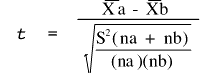
where : and are the arithmetic means for groups A and B, na and nb are the number of observations in groups A and B, and S² is the pooled within-group variance.

To compute the pooled within variance, we calculate the corrected sum of squares (SS) within each treatment group.

 

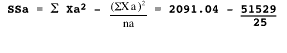
= 2091.04 - 2061.16 = 29.88

 

= 3038.28 - 3015.38 = 22.90

 

Then the pooled variance is

 

 

= 1.077

 

and,

 

= 5.814

 

This value of t has (na - 1) + (nb - 1) degrees of freedom. If it exceeds the tabular value of t (Table 3g-4) at a pre-determined probability level, we can reject the null hypothesis, and the difference between the two means would be considered statistically significant (greater than would be expected by chance if there is actually no difference).

In this case, the critical t value with 49 degrees of freedom at the 0.01 probability level is approximately 2.682. Since our sample is greater than this, the difference is significant at the 0.01 level and we can reject the null hypothesis.

 

The Paired t-Test

The previous description for the t-test assumed that the random samples are drawn from the two populations independently. However, there are some situations where the observations are paired. Analyzing paired data is done differently than if the two samples are independent. This modified procedure is known as a paired t-test. Most statistical software programs that perform the Student's t-test have options to select for either a paired or unpaired analysis.

 

Table 3g-4: Critical values of Student's t-distribution (2-tailed).

Degrees of Freedom	P=0.10	P=0.05	P=0.02	P=0.01	P=0.001	Degrees of Freedom
1	6.314	12.706	31.821	63.657	636.619	1
2	2.920	4.303	6.965	9.925	31.598	2
3	2.353	3.182	4.541	5.841	12.924	3
4	2.132	2.776	3.747	4.604	8.610	4
5	2.015	2.571	3.365	4.032	6.869	5
6	1.943	2.447	3.143	3.707	5.959	6
7	1.895	2.365	2.998	3.499	5.408	7
8	1.860	2.306	2.896	3.355	5.041	8
9	1.833	2.262	2.821	3.250	4.781	9
10	1.812	2.228	2.764	3.169	4.587	10
11	1.796	2.201	2.718	3.106	4.437	11
12	1.782	2.179	2.681	3.055	4.318	12
13	1.771	2.160	2.650	3.012	4.221	13
14	1.761	2.145	2.624	2.977	4.140	14
15	1.753	2.131	2.602	2.947	4.073	15
16	1.746	2.120	2.583	2.921	4.015	16
17	1.740	2.110	2.567	2.898	3.965	17
18	1.734	2.101	2.552	2.878	3.922	18
19	1.729	2.093	2.539	2.861	3.883	19
20	1.725	2.086	2.528	2.845	3.850	20
21	1.721	2.080	2.518	2.831	3.819	21
22	1.717	2.074	2.508	2.819	3.792	22
23	1.714	2.069	2.500	2.807	3.767	23
24	1.711	2.064	2.492	2.797	3.745	24
25	1.708	2.060	2.485	2.787	3.725	25
26	1.706	2.056	2.479	2.779	3.707	26
27	1.703	2.052	2.473	2.771	3.690	27
28	1.701	2.048	2.467	2.763	3.674	28
29	1.699	2.045	2.462	2.756	3.659	29
30	1.697	2.042	2.457	2.750	3.646	30
40	1.684	2.021	2.423	2.704	3.551	40
60	1.671	2.000	2.390	2.660	3.460	60
120	1.658	1.980	2.358	2.617	3.373	120

 

Study Guide

Additional Readings