(h). Inferential Statistics: Regression and Correlation

Introduction

Regression and correlation analysis are statistical techniques used extensively in physical geography to examine causal relationships between variables. Regression and correlation measure the degree of relationship between two or more variables in two different but related ways. In regression analysis, a single dependent variable, Y, is considered to be a function of one or more independent variables, X1, X2, and so on. The values of both the dependent and independent variables are assumed as being ascertained in an error-free random manner. Further, parametric forms of regression analysis assume that for any given value of the independent variable, values of the dependent variable are normally distributed about some mean. Application of this statistical procedure to dependent and independent variables produces an equation that "best" approximates the functional relationship between the data observations.

Correlation analysis measures the degree of association between two or more variables. Parametric methods of correlation analysis assume that for any pair or set of values taken under a given set of conditions, variation in each of the variables is random and follows a normal distribution pattern. Utilization of correlation analysis on dependent and independent variables produces a statistic called the correlation coefficient (r). The square of this statistical parameter (the coefficient of determination or r²) describes what proportion of the variation in the dependent variable is associated with the regression of an independent variable.

Analysis of variance is used to test the significance of the variation in the dependent variable that can be attributed to the regression of one or more independent variables. Employment of this statitical procedure produces a calculated F-value that is compared to a critical F-values for a particular level of statistical probability. Obtaining a significant calculated F-value indicates that the results of regression and correlation are indeed true and not the consequence of chance.

 

Simple Linear Regression

In a simple regression analysis, one dependent variable is examined in relation to only one independent variable. The analysis is designed to derive an equation for the line that best models the relationship between the dependent and independent variables. This equation has the mathematical form:

 

Y = a + bX

 

where, Y is the value of the dependent variable, X is the value of the independent variable, a is the intercept of the regression line on the Y axis when X = 0, and b is the slope of the regression line.

The following table contains randomly collected data on growing season precipitation and cucumber yield (Table 3h-1). It is reasonable to suggest that the amount of water received on a field during the growing season will influence the yield of cucumbers growing on it. We can use this data to illustate how regression analysis is carried out. In this table, precipitation is our independent variable and is not affected by variation in cucumber yield. However, cucumber yield is influenced by precipitation, and is therefore designated as the Y variable in the analysis.

 

Table 3h-1: Cucumber yield vs precipitation data for 62 observations.

 

Precipitation mm (X)	Cucumbers kilograms per m2 (Y)	Precipitation mm (X)	Cucumbers kilograms per m2 (Y)
22	.36	103	.74
6	.09	43	.64
93	.67	22	.50
62	.44	75	.39
84	.72	29	.30
14	.24	76	.61
52	.33	20	.29
69	.61	29	.38
104	.66	50	.53
100	.80	59	.58
41	.47	70	.62
85	.60	81	.66
90	.51	93	.69
27	.14	99	.71
18	.32	14	.14
48	.21	51	.41
37	.54	75	.66
67	.70	6	.18
56	.67	20	.21
31	.42	36	.29
17	.39	50	.56
7	.25	9	.13
2	.06	2	.10
53	.47	21	.18
70	.55	17	.17
6	.07	87	.63
90	.69	97	.66
46	.42	33	.18
36	.39	20	.06
14	.09	96	.58
60	.54	61	.42

 

S X = 3,050

= 49.1935

S Y = 26.62

= 0.4294

n = 62

 

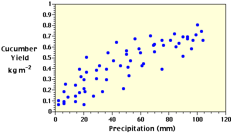
Often the first step in regression analysis is to plot the X and Y data on a graph (Figure 3h-1). This is done to graphically visualize the relationship between the two variables. If there is a simple relationship, the plotted points will have a tendancy to form a recognizable pattern (a straight line or curve). If the relationship is strong, the pattern will be very obvious. If the relationship is weak, the points will be more spread out and the pattern less distinct. If the points appear to fall pretty much at random, there may be no relationship between the two variables.

Figure 3h-1: Scattergram plot of the precipitation and cucumber yield data found in Table 3h-1. The distribution of the data points indicates a possible positive linear relationship between the two variables.

 

The type of pattern (straight line, parabolic curve, exponential curve, etc.) will determine the type of regression model to be applied to the data. In this particular case, we will examine data that produces a simple straight-line relationship (see Figure 3h-1). After selecting the model to be used, the next step is to calculate the corrected sums of squares and products used in a bivariate linear regression analysis. In the following equations, capital letters indicate uncorrected values of the variables and lower-case letters are used for the corrected parameters in the analysis.

 

The corrected sum of squares for Y:

S y² = S Y² -

= (0.36² + 0.09² + ... + 0.42²) - (26.62²) / 62

= 2.7826

 

The corrected sum of squares for X:

S x² = S X² -

= (22² + 6² + ... + 61²) - (3,050²) / 62

= 59,397.6775

 

The corrected sum of products:

S xy = S (XY) -

= ((22)(.36) + (6)(.09) + ... + (61)(.42)) - ((26.62)(3,050)) / 62

= 354.1477

 

As discussed earlier, the general form of the equation for a straight line is Y = a + bX. In this equation, a and b are constants or regression coefficients that are estimated from the data set. Based on the mathematical procedure of least squares, the best estimates of these coefficients are:

 

= (354.1477) / (59,397.6775) = 0.0060

 

a = Y - bX = 0.42935 - (0.0060)(49.1935) = 0.1361

 

Substituting these estimates into the general linear equation suggests the following relationship between the Y and X variables:

 

= 0.1361 + 0.0060X

 

where indicates that we are using an estimated value of Y.

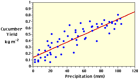
With this equation, we can estimate the the number of cucumbers (Y) from the measurements of precipitation (X) and describe this relationship on our scattergram with a best fit straight-line (Figure 3h-2). Because Y is estimated from a known value of X, it is called the dependent variable and X the independent variable. In plotting the data in a graph, the values of Y are normally plotted along the vertical axis and the values of X along the horizontal axis.

Figure 3h-2: Scattergram plot of the precipitation and cucumber yield data and the regression model best fit straight-line describing the linear relationship between the two variables.

 

Regression Analysis and ANOVA

A regression model can be viewed of as a type of moving average. The regression equation attempts to explain the relationship between the Y and X variables through linear association. For a particular value of X, the regression model provides us with an estimated value of Y. Yet, Figure 3h-2 indicates that many of the plotted values of the actual data are observed to be above the regression line while other values are found below it. These variations are caused either by sampling error or the fact that some other unexplained independent variable influences the individual values of the Y variable.

The corrected sum of squares for Y (i.e., S y²) determines the total amount of variation that occurs with the individual observations of Y about the mean estimate of . The amount of variation in Y that is directly related with the regression on X is called the regression sum of squares. This value is calculated accordingly:

 

Regression SS = = (354.1477)² / (59,397.6775) = 2.1115

 

As discussed above, the total variation in Y is determined by S y² = 2.7826. The amount of the total variation in Y that is not associated with the regression is termed the residual sum of squares. This statistical paramter is calculated by subtracting the regression sum of squares from the corrected sum of squares for Y (S y²):

 

Residual SS = S y² - Regression SS

= 2.7826 - 2.1115

= 0.6711

 

The unexplained variation can now be used as a standard for testing the amount of variation attributable to the regression. Its significance can be tested with the F test from calculations performed in an Analysis of Variance table.

 

Source of variation	df 1	SS	MS 2
Due to regression	1	2.1115	2.1115
Residual (unexplained)	60	0.6711	0.0112
Total	61	2.7826	-

1 There were 62 values of Y analyzed and therefore n = 62. The total sum of squares degrees of freedom (df) is determined as n-1 or 61. The regression of Y on X has 1 degree of freedom. The residual or unexplained degrees of freedom is determined by subtracting regression df (1) from total sum of squares df (61).

2 MS is calculated as SS / df.

Using the Analysis of Variance procedure, the regression is tested by determining the calculated F statistic:

 

F = (Regression MS) / (Residual SS) = (2.1115) / (0.0112) = 188.86

 

To test this statistic we use a table of F to determine a critical test value for a probability of 0.01 or 1% (this relationship can occur by chance only in 1 out 100 cases) and with 1,60 degrees of freedom. According to the table the critical test value is 7.1. In this test, the relationship is deemed significant if the calculated F statistic is greater than the critical test value. This regression is statistically significant at the 0.01 level because 188.86 is greater than 7.1.

Caution must be taken when interpreting the results of regression. In our example, we found a significant relationship between precipitation and cucumber yield. However, this conclusion may not be the result of a causal relationship between the two variables. A third variable that is directly associated to both precipitation and cucumber yield may be confounding the interpretation of the analysis. Absolute verification of associations between variables can only be confirmed with experimental manipulation.

 

Coefficient of Determination

To measure how strong the correlation is between the two variables, we can determine the amount of the total variation in Y that is associated with the regression model. This ratio is sometimes called the coefficient of determination and is represented by the symbol r². The value of the coefficient of determination ranges from 1.00 to 0.00. The calculated coefficient of determination from the data set above was 0.76 or 76% (as calculated below). This value suggests that 76% of the variation in Y was associated with the change seen X from the data set observations.

 

Coefficient of determination = (Regression SS) / (Total SS)

= (2.1115) / (2.7826) = 0.7588

 

Correlation Coefficient

Another useful regression statistic that measures the strength of the correlation between to variables is the correlation coefficient.This statistic is often represented by the symbol "r" and is determined by taking the square-root of the coefficient of determination. The value of the correlation coefficient ranges from 1.00 to -1.00. A value of 0.0 indicates that there is absolutely no relationship between the X and Y variables. The strength of the relationship between the X and Y variables increases as the value of r approaches 1.00 and -1.00. Perfect correlation occurs if r equals either 1.00 (perfect positive) or -1.00 (perfect negative). Positive correlation coefficients indicate that an increase in the value of the X variable results in an increase in the value of the Y variable. Negative correlation coefficients indicate that an increase in the value of the X variable results in a decrease in the value of the Y variable.

Study Guide

Additional Readings